Outline:
Range
Border
Zero axes
Key
Tics
Major tics
Minor tics
Nomirror and second tics
Other options for tics
Grid
Want only the plot?
Title, key title, and lable
Title
Key title
Label
Arrow
Resolution
3D Plot general
Scaling
Size ratio
Tics level
Log scale
Parameterizing
Parametric
Polar
Border
Zero axes
Key
Tics
Major tics
Minor tics
Nomirror and second tics
Other options for tics
Grid
Want only the plot?
Title, key title, and lable
Title
Key title
Label
Arrow
Resolution
3D Plot general
Scaling
Size ratio
Tics level
Log scale
Parameterizing
Parametric
Polar
Data plot
Basics
Vector
Bar graph
Line and point styles
Multiple columns data plot
Multiplot
For CSV files
For Fortran high precision data
Error bars
Candle chart
3D data plot
Other tips
Define a function
Plot with complex variables
Tertiary operator
Skip data values
Gnuplot as a calculator
Timestamp
Data fitting
Data plot
Basics
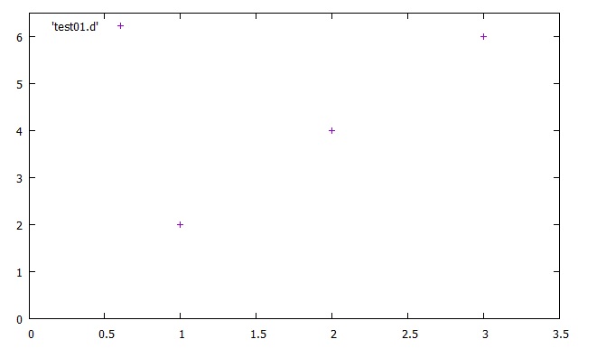
In all the previous sections, we used the built-in functions of gnuplot, but you can also plot extrernal data files. For example, you have the following forrmatted data saved as test01.d:
# X Y
1.0 2.0
2.0 4.0
3.0 6.0
The symbol, #, can comment out; in a word, gnuplot ignores the whole referred line. Now, let's plot this by gnuplot:
1.0 2.0
2.0 4.0
3.0 6.0
gnuplot> plot [0:3.5] [0:6.5] 'test01.d'
Note that you MUST use quotations or double quotations for the file name in the command line.
You also have to locate the folder that the file exists for gnuplot.
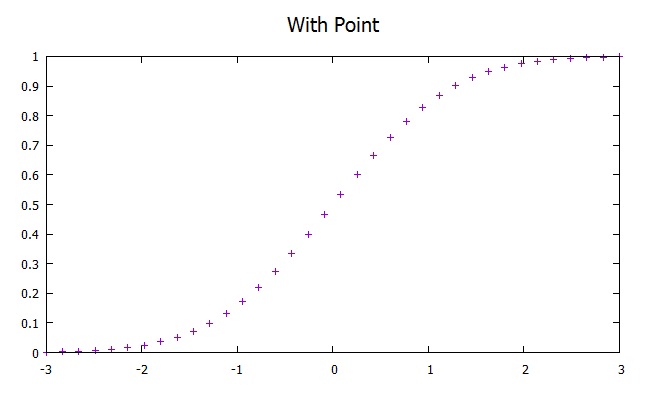
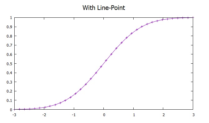
You can specify the sizes, colors and shapes of the plotted points. The line connecting between points can also be displayed. You just type "with line", or "with linespoint" after the plot command. They can be abbreviated as "w l" and "w lp." All the options are listed as follows:
gnuplot> plot 'example.d' w p # Plot with points
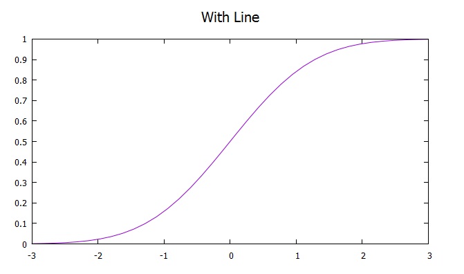
gnuplot> plot 'example.d' w l # Plot with lines
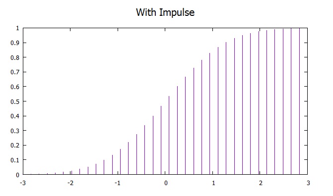
gnuplot> plot 'example.d' w i # Plot with impulses
gnuplot> plot 'example.d' w d # Plot with dots (tyny little points)
gnuplot> plot 'example.d' w lp # Plot with lines and points
gnuplot> plot 'example.d' w l # Plot with lines
gnuplot> plot 'example.d' w i # Plot with impulses
gnuplot> plot 'example.d' w d # Plot with dots (tyny little points)
gnuplot> plot 'example.d' w lp # Plot with lines and points
Vector
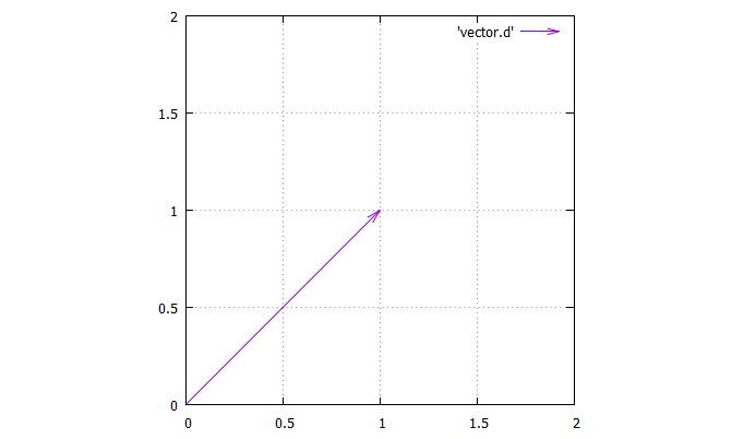
There is also a convenient option that is "plot with vector." In order to plot a set of data as a vector, you need 4 values. The first two are x and y coordinates of the start point. The next two are x and y components; in other words, they are lengths of x and y. Take a look at the following data file (vector.d):
# Start Length
# (x, y) (x, y)
0.0 0.0 1.0 1.0
Then, command as follows:
# (x, y) (x, y)
0.0 0.0 1.0 1.0
gnuplot> plot 'vector.d' w vector
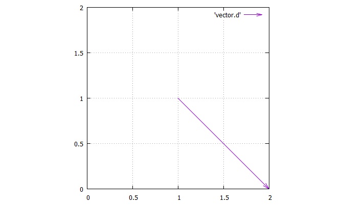
Let's look at another example.
1.0 1.0 1.0 -1.0
The start point is (1, 1); the x component takes length of 1 in the positive direction; then
the y component takes length of 1 in the negative direction. Make sure this with the output figure:
Bar graph
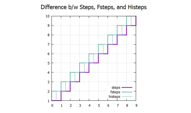
There are several options to plot the data with a bar graph. The "box" option is a simple bar graph, but the "step" options can produce variations of steps to be plotted.
gnuplot> plot 'example.d' w boxes # Plot with boxes (cannot be abbreviated)
gnuplot> plot 'example.d' w steps # Plot with steps (cannot be abbreviated)
gnuplot> plot 'example.d' w fsteps # Plot with steps (cannot be abbreviated)
gnuplot> plot 'example.d' w histeps # Plot with steps (cannot be abbreviated)
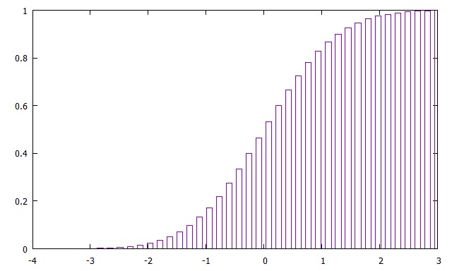
Let's plot erf.d with "box" option.
gnuplot> plot 'example.d' w steps # Plot with steps (cannot be abbreviated)
gnuplot> plot 'example.d' w fsteps # Plot with steps (cannot be abbreviated)
gnuplot> plot 'example.d' w histeps # Plot with steps (cannot be abbreviated)
gnuplot> plot 'erf.d' w boxes
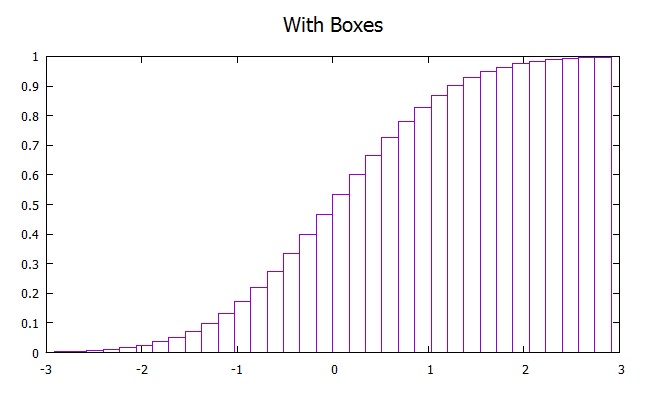
gnuplot> set boxwidth 0.1
gnuplot> plot 'erf.d' w boxes
gnuplot> plot 'erf.d' w boxes
Then, plot step.d with three different options of "steps" in one frame as follows:
gnuplot> plot [0:9][1:10] 'step.d' w steps, 'step.d' w fsteps, 'step.d' w histeps
Note that you may have to adjust the ranges and other settings to have exactly the same as the following.
Line and point styles
You may need a thicker line or a larger size of point for some reason. Here are the options:
gnuplot> plot 'example.d' lw 2 # Specify the line width
gnuplot> plot 'example.d' lt 3 # Specify the line color (must be done before linewidth)
gnuplot> plot 'example.d' pt 3 # Specify the point type
gnuplot> plot 'example.d' ps 4 # Specify the point size
gnuplot> plot 'example.d' dt 1 # Specify the dash type
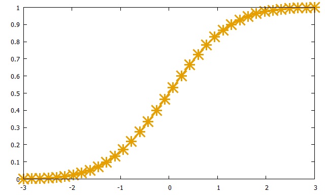
Let's plot some example with erf.d.
gnuplot> plot 'example.d' lt 3 # Specify the line color (must be done before linewidth)
gnuplot> plot 'example.d' pt 3 # Specify the point type
gnuplot> plot 'example.d' ps 4 # Specify the point size
gnuplot> plot 'example.d' dt 1 # Specify the dash type
gnuplot> plot 'erf.d' lt 4 lw 3 pt 3 ps 3 w lp
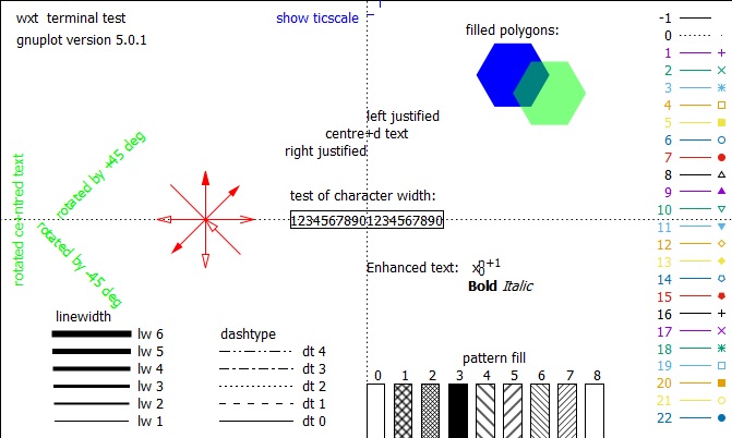
gnuplot> test
Multiple data columns
Suppose you have the following data (bessel.d):
0.000000 0.000000 0.000000 0.000000
0.166667 0.083044 0.003464 0.000096
0.333333 0.164363 0.013761 0.000766
0.500000 0.242268 0.030604 0.002564
0.666667 0.315155 0.053526 0.006003
0.833333 0.381529 0.081890 0.011542
1.000000 0.440051 0.114903 0.019563
1.166667 0.489557 0.151643 0.030362
1.333333 0.529095 0.191076 0.044134
1.500000 0.557937 0.232088 0.060964
1.666667 0.575599 0.273510 0.080825
1.833333 0.581853 0.314153 0.103571
2.000000 0.576725 0.352834 0.128943
2.166667 0.560498 0.388412 0.156570
2.333333 0.533701 0.419812 0.185977
2.500000 0.497094 0.446059 0.216600
2.666667 0.451651 0.466299 0.247798
2.833333 0.398533 0.479825 0.278867
3.000000 0.339059 0.486091 0.309063
...
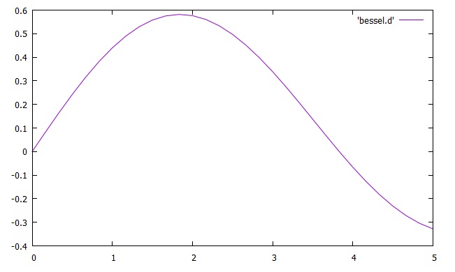
The default of the plot command picks out the first and second as x and y values.
0.166667 0.083044 0.003464 0.000096
0.333333 0.164363 0.013761 0.000766
0.500000 0.242268 0.030604 0.002564
0.666667 0.315155 0.053526 0.006003
0.833333 0.381529 0.081890 0.011542
1.000000 0.440051 0.114903 0.019563
1.166667 0.489557 0.151643 0.030362
1.333333 0.529095 0.191076 0.044134
1.500000 0.557937 0.232088 0.060964
1.666667 0.575599 0.273510 0.080825
1.833333 0.581853 0.314153 0.103571
2.000000 0.576725 0.352834 0.128943
2.166667 0.560498 0.388412 0.156570
2.333333 0.533701 0.419812 0.185977
2.500000 0.497094 0.446059 0.216600
2.666667 0.451651 0.466299 0.247798
2.833333 0.398533 0.479825 0.278867
3.000000 0.339059 0.486091 0.309063
...
gnuplot> plot 'bessel.d' w l
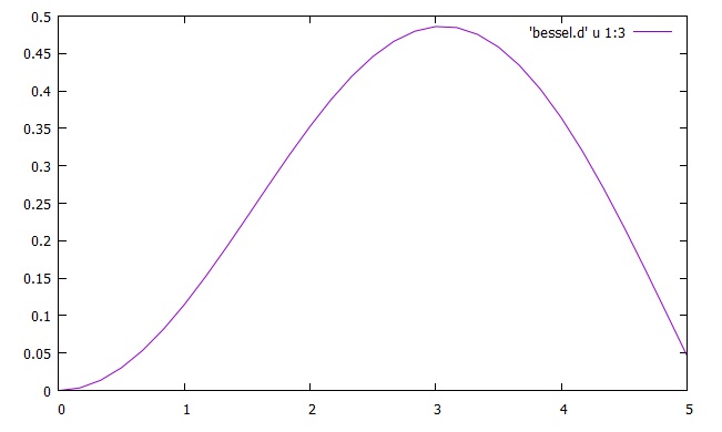
If you need to plot the first and third as x and y, specify with "using" command.
gnuplot> plot 'bessel.d' u 1:3 w l
The option, "u", represents "using", and "1:3" specifies the first and third columns in the data file.
The "using" command MUST be used before "with lines" command.
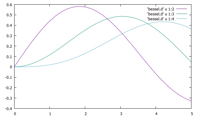
gnuplot> plot 'bessel.d' u 1:2 w l, 'bessel.d' u 1:3 w l, 'bessel.d' u 1:4 w l
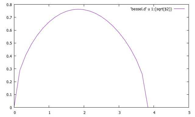
You can modify data columns in command lines. In the "using " command, specify the number of column. Say, pick out the second column, and operate square root on this.
gnuplot> plot 'bessel.d' u 1:(sqrt($2)) w l
Here is the plot with the first column and square root of the second column.
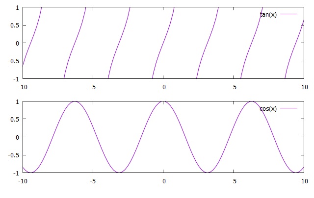
Multiplot
You can display multiple coordinates in single output. Just follow this instruction:
gnuplot> set multiplot layout 2,1
multiplot> plot tan(x)
multiplot> plot cos(x)
You will obtain the following output:
multiplot> plot tan(x)
multiplot> plot cos(x)
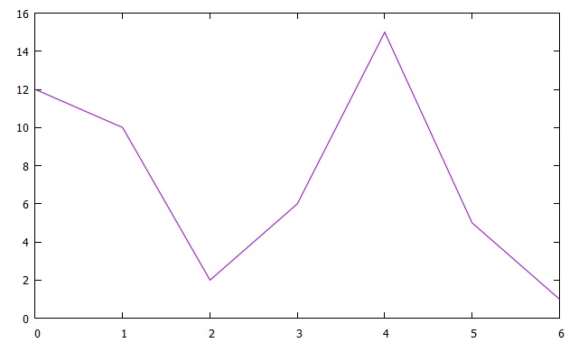
For CSV files
The data in CSV files or any data separated by commas are not plotted properly in gnuplot. For example, (csv.d)
12,6
10,1
2,11
6,8
15,7
5,6
1,4
In order to ignore commas for the proper plot, you should use the following command:
10,1
2,11
6,8
15,7
5,6
1,4
gnuplot> set datafile separator ","
Then, you have
For Fortran high precision data
If the data calculated from a Fortran program are double or quadrruple precision, use the following command:
gnuplot> set datafile fortran
This enables a special check for reading data sets.
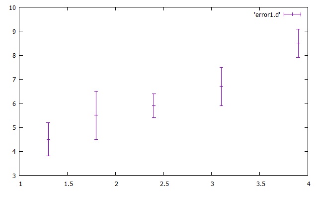
Error bars
A typical plot with error bar requires 3-column of data. (error1.d)
# x y error
1.3 4.5 0.7
1.8 5.5 1.0
2.4 5.9 0.5
3.1 6.7 0.8
3.9 8.5 0.6
As shown above, the third column expresses the range of error. Let's plot this with the error bar of
y axis.
1.3 4.5 0.7
1.8 5.5 1.0
2.4 5.9 0.5
3.1 6.7 0.8
3.9 8.5 0.6
gnuplot> plot 'error1.d' w yerrorbars
gnuplot> plot 'error1.d' w xerrorbars
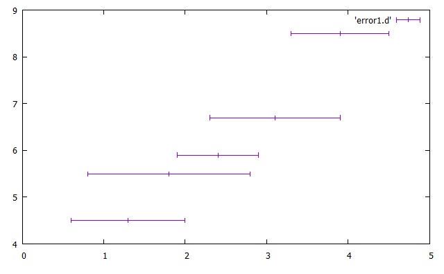
Then, the following is plotted with the bar graph:
gnuplot> plot 'error1.d' w boxerrorbars
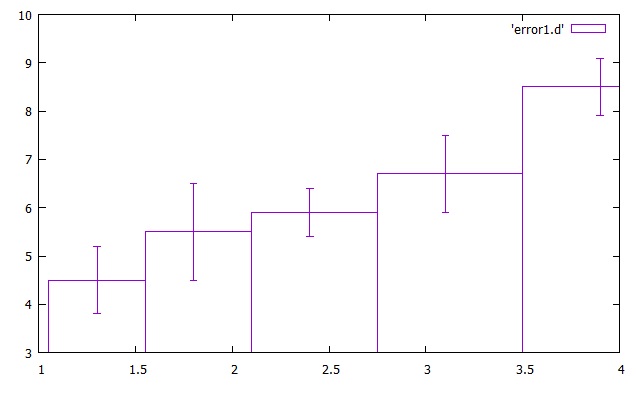
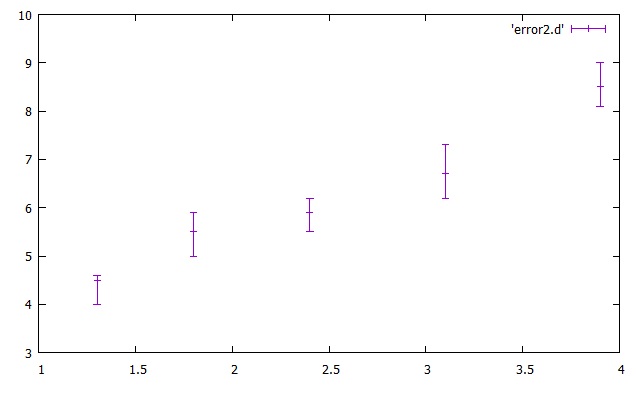
# x y error
1.3 4.5 4.0 4.6
1.8 5.5 5.0 5.9
2.4 5.9 5.5 6.2
3.1 6.7 6.2 7.3
3.9 8.5 8.1 9.0
Then, command as follows:
1.3 4.5 4.0 4.6
1.8 5.5 5.0 5.9
2.4 5.9 5.5 6.2
3.1 6.7 6.2 7.3
3.9 8.5 8.1 9.0
gnuplot> plot 'error2.d' w yerrorbars
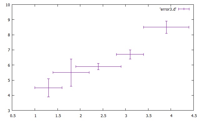
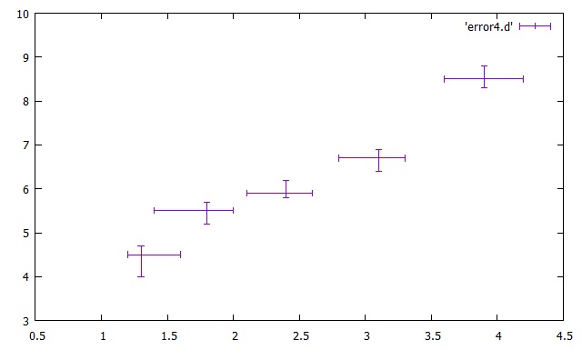
You can have both x- and y-error bars with a 4-column set of data. (error3.d)
# x y error
1.3 4.5 0.3 0.6
1.8 5.5 0.4 0.9
2.4 5.9 0.5 0.2
3.1 6.7 0.3 0.3
3.9 8.5 0.5 0.4
1.3 4.5 0.3 0.6
1.8 5.5 0.4 0.9
2.4 5.9 0.5 0.2
3.1 6.7 0.3 0.3
3.9 8.5 0.5 0.4
gnuplot> plot 'error3.d' w xerrorbars
# x y error
1.3 4.5 1.2 1.6 4.0 4.7
1.8 5.5 1.4 2.0 5.2 5.7
2.4 5.9 2.1 2.6 5.8 6.2
3.1 6.7 2.8 3.3 6.4 6.9
3.9 8.5 3.6 4.2 8.3 8.8
1.3 4.5 1.2 1.6 4.0 4.7
1.8 5.5 1.4 2.0 5.2 5.7
2.4 5.9 2.1 2.6 5.8 6.2
3.1 6.7 2.8 3.3 6.4 6.9
3.9 8.5 3.6 4.2 8.3 8.8
gnuplot> plot 'error4.d' w xyerrorbars
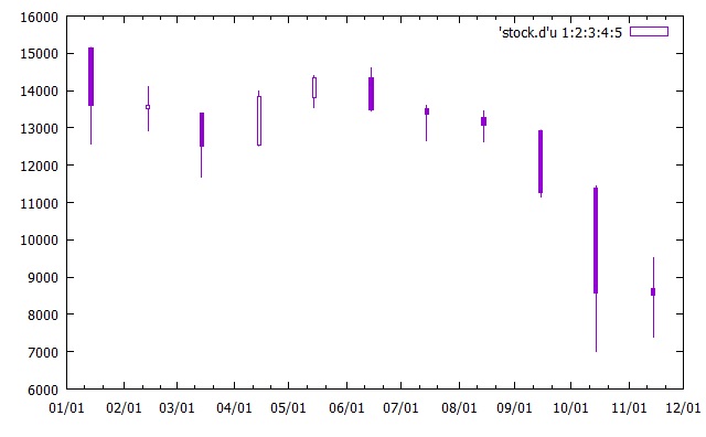
Candle chart
If you have a set of data for stock exchange, you can plot it with candle charts. The data must be 5-column, which are date, open, high, low, and close, respectively. Here is an example, (stock.d):
01-15-2008 15155.73 15156.66 12572.68 13592.47
02-15-2008 13517.74 14105.47 12923.42 13603.02
03-15-2008 13412.87 13413.63 11691.00 12525.54
04-15-2008 12539.80 14003.28 12521.84 13849.99
05-15-2008 13802.59 14392.53 13540.68 14338.54
06-15-2008 14342.96 14601.27 13453.35 13481.38
07-15-2008 13514.86 13603.31 12671.34 13376.81
08-15-2008 13276.57 13468.81 12631.94 13072.87
09-15-2008 12936.81 12940.55 11160.83 11259.86
10-15-2008 11396.61 11456.64 6994.90 8576.98
11-15-2008 8702.77 9521.24 7406.18 8512.27
Then, enter as follows in the command lines:
02-15-2008 13517.74 14105.47 12923.42 13603.02
03-15-2008 13412.87 13413.63 11691.00 12525.54
04-15-2008 12539.80 14003.28 12521.84 13849.99
05-15-2008 13802.59 14392.53 13540.68 14338.54
06-15-2008 14342.96 14601.27 13453.35 13481.38
07-15-2008 13514.86 13603.31 12671.34 13376.81
08-15-2008 13276.57 13468.81 12631.94 13072.87
09-15-2008 12936.81 12940.55 11160.83 11259.86
10-15-2008 11396.61 11456.64 6994.90 8576.98
11-15-2008 8702.77 9521.24 7406.18 8512.27
gnuplot> set xdata time #optional to express dates
gnuplot> set timefmt "%m-%d-%Y" #optional to express dates
gnuplot> plot 'stock.d' u 1:2:3:4:5 w candlesticks
gnuplot> set timefmt "%m-%d-%Y" #optional to express dates
gnuplot> plot 'stock.d' u 1:2:3:4:5 w candlesticks
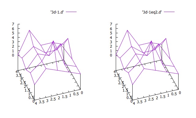
3D data plot
For one of the 3D-plot data, you can have the following, (3d-1.d):
0
0
0
3
0
1
1
4
1
1
2
7
2
1
1
3
3
3
3
5
0
1
0
1
0
This will be a 3D surface plot if you use "splot" command. The data above are values for z axis. In other words, this
is equivalent with the following data (3d-1eq2.d):
0
0
3
0
1
1
4
1
1
2
7
2
1
1
3
3
3
3
5
0
1
0
1
0
#x y z
0 0 0
1 0 0
2 0 0
3 0 3
4 0 0
0 1 1
1 1 1
2 1 4
3 1 1
4 1 1
0 2 2
1 2 7
2 2 2
3 2 1
4 2 1
0 3 3
1 3 3
2 3 3
3 3 3
4 3 5
0 4 0
1 4 1
2 4 0
3 4 1
4 4 0
The both files can generate the same plot as follows:
0 0 0
1 0 0
2 0 0
3 0 3
4 0 0
0 1 1
1 1 1
2 1 4
3 1 1
4 1 1
0 2 2
1 2 7
2 2 2
3 2 1
4 2 1
0 3 3
1 3 3
2 3 3
3 3 3
4 3 5
0 4 0
1 4 1
2 4 0
3 4 1
4 4 0
gnuplot> set multiplot layout 1,2
multiplot> splot '3d-1.d' w l
multiplot> splot '3d-1eq2.d' w l
multiplot> splot '3d-1.d' w l
multiplot> splot '3d-1eq2.d' w l
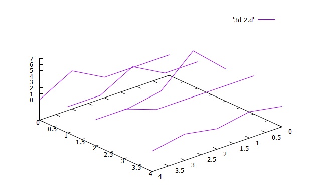
How about if you put a double space for each block? (3d-2.d)
#x y z
0 0 0
1 0 0
2 0 0
3 0 3
4 0 0
0 1 1
1 1 1
2 1 4
3 1 1
4 1 1
0 2 2
1 2 7
2 2 2
3 2 1
4 2 1
0 3 3
1 3 3
2 3 3
3 3 3
4 3 5
0 4 0
1 4 1
2 4 0
3 4 1
4 4 0
0 0 0
1 0 0
2 0 0
3 0 3
4 0 0
0 1 1
1 1 1
2 1 4
3 1 1
4 1 1
0 2 2
1 2 7
2 2 2
3 2 1
4 2 1
0 3 3
1 3 3
2 3 3
3 3 3
4 3 5
0 4 0
1 4 1
2 4 0
3 4 1
4 4 0
gnuplot> splot '3d-2.d' w l
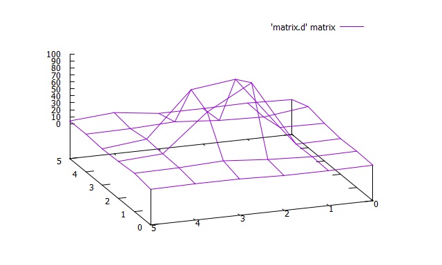
Suppose you have a set of data in a matrix form (matrix.d).
1 2 1 4 9 0
0 1 0 5 1 2
0 4 95 81 3 1
2 9 60 73 8 1
2 6 7 9 5 9
1 5 3 2 4 4
The rows and columns correspond to x and y coordinates. Use the matrix option to plot this.
0 1 0 5 1 2
0 4 95 81 3 1
2 9 60 73 8 1
2 6 7 9 5 9
1 5 3 2 4 4
gnuplot> splot 'matrix.d' matrix w l
| Previous page | Next page |